Introduction

Many Computer Science projects suffers from lack of theoretical information behind ideas which they try to implement. This project is in fact different because has been built on simple idea that we would like to share not only code but also ideas behind it. This part of our web page contains basic explanation of several topic related to curvature and its application to smoothing of polyhedral meshes. The plan of this page is as fallows at first we will discuss in short curvature in general, after that we introduce notation of abstract polyhedral mesh to finally talk about discrete mean curvature and flow based on it. Moreover the last part deals with drawbacks of mean curvature flow.

Curvature

Intuitive definition of curvature is how much something departs from being flat or straight. We can also define positive curvature e.g. sphere or negative e.g. saddle surface and also zero curvature when we talk e.g. about plane. See figure 1. In case of curves we can define curvature e.g. by osculating circle but this definition of curvature can not be used for surfaces.

Figure 1. From left to right. Positive, negative and zero curvature. Image comes from thephysicsmill.com.

Curvature of 3-dimensional differentiable surfaces can be defined in several ways e.g. Gaussian curvature or mean curvature. In continuous space curvature at each point p of surface is defined by two principal curvatures. One can choose a normal vector at p and define a normal plane which goes through it. Each defined in this way normal plane will cut the surface in a plane curve. Each plane curve defined by different normal plane will have in general different curvature. Two principal curvatures $\kappa$₁, $\kappa$₂ are the maximal and minimal curvatures defined by normal planes around normal vector. We can better understand this idea by taking a look on figure 2 which presents a surface with two principal curvature planes - normal planes.

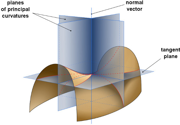
According to figure 2 mean curvature is defined as:

And Gaussian curvature as:

Right now we talk a bit more about mean curvature which will be exhaustively used in the subsequent parts. Mean curvature in general is a gradient of area $\vec{(H)} = H \vec{n} = \nabla area$ and contains information how much the surface area changes at constant speed along the surface normals and in fact tell us how to increase in an efficient way surface area, or decrease if we inverse the gradient.

Meshes

Before we will talk about mean curvature of polyhedral meshes we have to define them and give some important condition under there will be possible to calculate mean curvature. Instead of speaking about any specific mesh we will define an abstract one and we give set of conditions under any general mesh is well defined from the perspective of future discussion. Also in this place is good to add that because we are interested only in meshes with whom computers can deal - so we will skip some general properties of abstract meshes like infinitely big set of vertices.

1. Mesh is build from finite set of vertices - V where we will denote one vertex by p_index
2. All vertices are connected by unordered edges which whole set will be denoted by E and particular edge denoted by e = (p_i, p_j) = (p_j, p_i) where p_i $\neq$ p_j. We assume that the number of edges which go through one vertex is finite and because we assumed in point 1 that set V is also finite therefore set E is also finite.
3. We will introduce a set F which contains closed paths build from distinct vertices (p₁, p₂, …, p_n, p₁) where p_i, p_i+1 form an edge. We will call these closed paths faces.

Conditions:

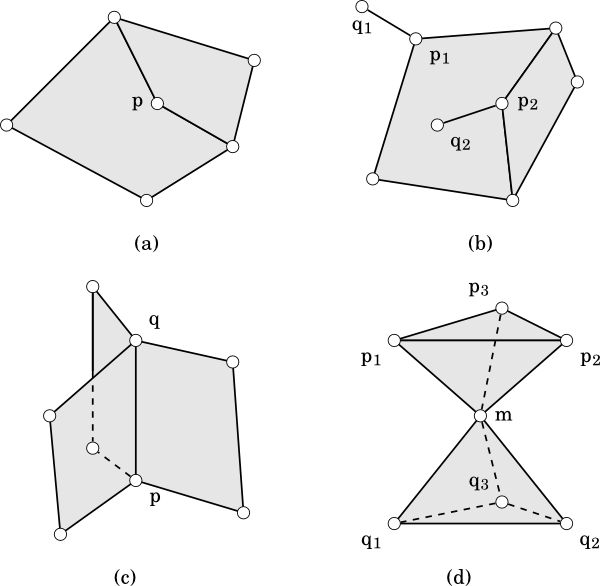
1. Through one vertex we can define 3 or more edges when vertex belongs to internal part of mesh or 2 when it belongs to boundary of mesh. (counter-example - figure 3. (a and b))
2. Each edge is incident to 2 faces when its an internal edge or only one when edges is a boundary one. (counter-example - figure 3. (b and c)) In this case mesh is not 2-manifold and we are not interested in fallowed parts in this degenerated case.
3. Each face has at least three edges. By simplification we will work in fallowed parts with faces whose $dim(f) = 3$ - triangular faces.
4. Each point belongs only to the one close mesh. This means that we can not have e.g. two close meshes connected by one point. (counter-example - figure 3. (d))

Discrete mean curvature

Discrete mean curvature is defined at vertices of polyhedral mesh instead of points of surface and takes into account curvature defined on edges and area of part of mesh contains given vertex.

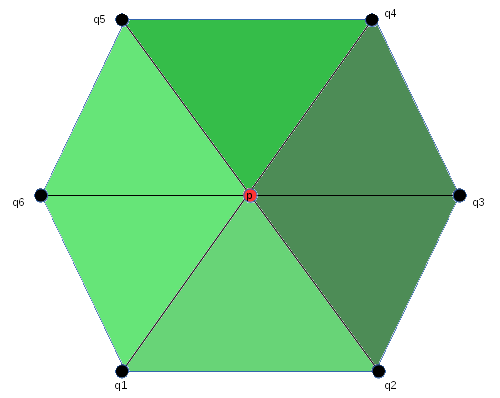
Where star of p is presented by figure 4 and is defined by for given vertex - p by all faces and edges which contain it.

Below formula defines mean curvature vector in details

where:

is a normal to edge defined by normals of adjacent faces which are defined as

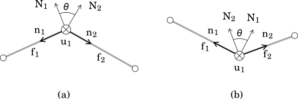
and angle $\theta$

This angle is defined between two adjacent normals to faces as presented by figure 5.

In fact this definition is an analog of continuous one. As was said above mean curvature vector gives information how to efficiently increase area. But we can change its direction to efficiently decrees area and therefore evolve our mesh by moving given vertex by inverted mean curvature vector. And this is exactly what mean curvature flow does. We can also add a time which allows to “jump” to particular evolved mesh. So final formula for mean curvature flow is as fallow:

In “Media” sub-page you can find several movies which presents evolving of different kind of meshes by mean curvature flow.

Boundary case

Above part of this page deals only with close polyhedral meshes, but we can still define mean curvature flow for non-close surfaces. Figure 6 presents start of p which is on surface boundary. In this case there is no notation of angle $\theta$ as before since we can not define it for all edges and therefore we use another strategy.

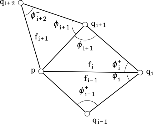
Below formula define mean curvature vector when vertex belongs to the boundary:

which is equal to

And right now we can see a link between both definitions.

Drawbacks of mean curvature flow

In general decreasing of area is a natural choice to remove bumps and noise from mesh. But as we will see this is not always true in case of mean curvature flow. In sub-page media there are several movies which presents mean curvature flow of several meshes but there is no sphere. Some people may think we would not add it because is obvious that it should evolve to point. At the beginning we thought same. Below movie presents interesting behavior of mean curvature flow.

As we see we do not get any excepted result. Also some of you may noticed that in case of Stanford bunny or dragon result is also not so good - mesh is not really “smoother”. Next movie shows in comparison Laplacian smoothing with cotangent weights(in some sense is same as mean curvature flow) and also to see non-regularity at first mean curvature map was calculated and also presented as different colors.

At first you can see that mean curvature map is not really uniform. We have some region with higher and lower curvature - differences in color. But we have to say that is proven that it’s impossible to create a polyhedral mesh which will be a real uniform sphere so these results are more and less predicted.

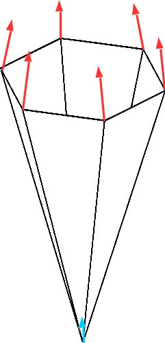
Also once again you can see that sphere is not evolving to point. Explanation of this problem in sense of mean curvature is that because our mean curvature vector is constant and we have two different regions with smaller and bigger curvature thus some of stars of p contains 5 and other 6 adjacent edges. As we saw on the movie some points are moving faster and some slower and if we take a closer look we can see that these vertices which are included in 5 adjacent edges are moving slower and creates spikes. This behavior is presented by figure 7 where spike is prescribed as a cone. In this case of figure 7 to vertex p are adjacent six edges but all other vertices which creates these edges have bigger starts and therefore they are moving faster also from these reasons star of given vertex is stretched and going to line.

Before we said that mean curvature flow is a solution to decrees area in most efficient way but we have to keep in mind that this not always mean to move vertex inwards. Figure 8 presents hypothetical case when after evolving area decreases but we ended-up with line and we did not smoother our surface.

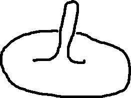
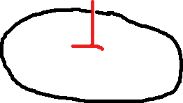
This implies that mean curvature flow is good only for regular polyhedrons. But if we are looking for more general solutions we should use e.g. Willmore flow. Right now we do not want to give any explanation of Willmore flow but you can take a look at below movie which presents conformal Willmore flow to see what we are talking about. People which are interested in the definition of discrete Willmore flow should take a look on (3).

References

1. Introduction à la géométrie différentielle discrète, P. Romon, 2014 - link
2. Polyhedral Surfaces of Constant Mean Curvature, K. Polthier, 2002 - link
3. Discrete Willmore flow, A. Bobenko and P. Schröder, 2005 - link